(v13) Calibration interpolation arrays

This page applies to Harlequin v13.1r0 and later; both Harlequin Core and Harlequin MultiRIP.

A few terms used in the explanation of calibration follow:

Calibration is generally done by printing a test strip, measuring the patches with a densitometer, and entering the resulting measured values . The RIP compares these with the Desired values or Patch values it used to produce the test strip.

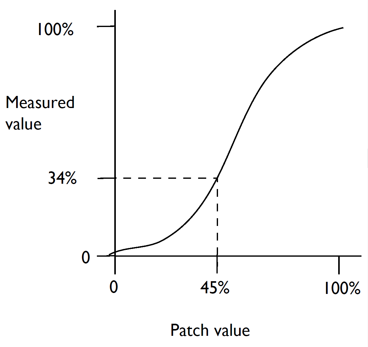
In principle, the function from Patch value to Measured value can be represented by a graph, which might look like this curve:

This graph is what you can see in the Calibration Edit dialog of the GUI version of the RIP. The dotted line shows that a Patch value of 45% produces a Measured value of 34% in this example. The shape of the graph depends on the measurement system chosen.

In reality when a job asks for a certain value it means a ScriptWorks Nominal Value (SNV), not a Measured value. To simplify printing jobs, the RIP actually stores the SNV (which is independent of the measurement system), rather than the Measured value, as part of the calibration process. It finds the SNV from the Measured value by using the conversion tables in the profile.

The RIP also converts the Patch value to the NDC value, (the conversion depends on whether you are editing in calibrated or uncalibrated mode and on the default curve). In other words, the RIP works out what NDC was actually used to print each Patch value. The calculation depends on what calibration if any was in force at the time the target was printed.

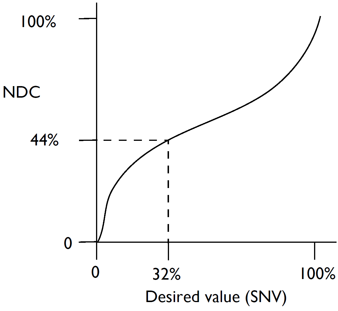
Therefore, rather than storing Measured values to Patch values, straight from the Calibration Edit dialog of the GUI version of the RIP, it actually stores SNV to NDC values, as shown in the following graph. As you can see the RIP has also flipped the graph round to get an NDC to send to the printer from a given desired value .

In the case of an uncalibrated edit with a linear default curve, this graph will be the same as the one above, but flipped round.

The graph above is in effect the combined calibration set and default curve. The default curve comes from a linearization profile of the output device. If the default curve is linear, the graph above equals the calibration set curve, as the default curve has no effect.

Conceptually therefore the RIP stores SNV to NDC values, (as it did literally in the old-style calibration set curves). Rather than storing the default curve combined with the day-to-day calibration data, this is kept separate, and the above graph is in practice stored as two graphs, that is SNV to SGV, (the new style calibration set curve), and SGV to NDC, (the default curve).

The next two diagrams show how the RIP uses these two graphs when printing a job in order to find out what NDC to send to the printer for a given desired value:

First the RIP uses the calibration set curve to get a corrected lookup value or (SGV) from a given desired value :

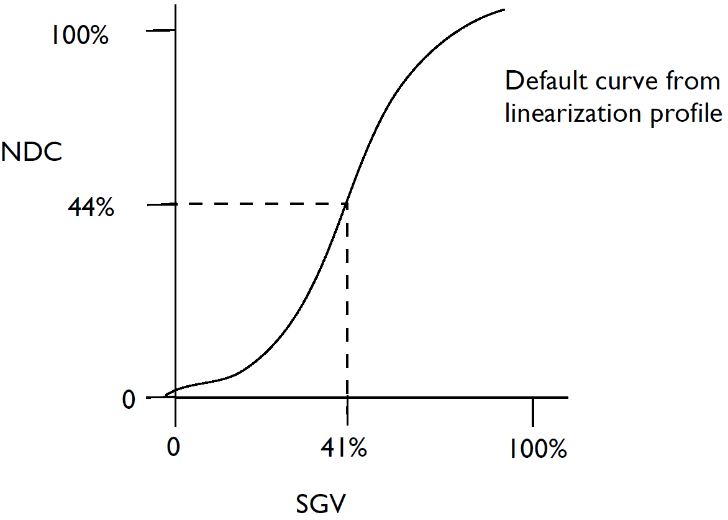
Now the default curve for the output device is applied. The default curve comes from the profile of the output device and is applied to the SGV found from the calibration set curve. This gives an NDC which is the actual value the RIP must supply to the printer.

In summary, if a job using this calibration asks for a tint of 32%, the NDC sent to the printer ise 44%.

In practice, the RIP only has measurements at some finite set of data points. However, it is good enough to interpolate between adjacent points to get the values in between. The RIP applies a linear interpolation function. Thus, taking the same case as above and supposing that few samples are measured, the actual calibration set curve applied would look like the solid line in the following graph:

Similarly, the default curve from the profile really consists of straight-line segments, (though not necessarily with the same number of points).

The RIP has built-in support for interpolation. In several places, an interpolation array can be given.

In the dictionary form of the calibration set, the interpolation arrays can themselves consist of two arrays. In this case the first array relates SNV to SGV value and the second array relates SGV to NDC, see Colorant subdictionaries (N-color calibration). If there is only one array present, it effectively relates SNV to NDC values.

You can think of this as each interpolation array or subarray relating a desired value to an actual value which you either send to the printer (NDC) or use as an input to another array.

Interpolation arrays must follow these rules:

• There must be an even number of entries.
• The first number of the first pair must be 0.0. The second is also usually 0.0.
• The first number of the last pair must be 1.0. The last number is also usually 1.0.
• The first number of each pair must be larger than the first number of the previous pair. For example, the graph above might be represented by the following interpolation array:

[0.0 0.0 .13 .30 .43 .52 .78 .65 .96 .83 1.0 1.0]

This is a contrived example for illustration only; a practical example would have more points, and probably be different in other ways.